SQL for Data Analysis - The Data Alchemist

Introduction: Why SQL is the #1 Skill for Data Analysts

Here’s a hard truth: You cannot be an effective data analyst without SQL.

Not Python. Not Tableau. Not Power BI. SQL.

Why? Because every single dataset in the real world lives in a database. Every dashboard you’ll ever build pulls from SQL queries. Every insight you’ll present started with someone asking a question of structured data. And that question—that’s answered with SQL.

This guide isn’t about teaching you SQL syntax. You can learn that from any tutorial. This guide is about teaching you to think like a data analyst using SQL—to write queries that are fast, efficient, and actually answer business questions.

SQL for Software Development vs. SQL for Data Analysis

This distinction matters because it changes everything about how you approach the language.

Aspect	Software Development SQL	Data Analysis SQL
Primary Goal	Insert/Update/Delete data reliably	Extract & analyze data insights
Query Focus	Small, fast queries returning 1-100 rows	Large, aggregated queries returning thousands of rows
Complexity	Transactions, constraints, data integrity	Joins, window functions, aggregations, subqueries
Optimization Focus	Data consistency & transaction speed	Query speed & result clarity
Most Used Commands	INSERT, UPDATE, DELETE	SELECT, JOIN, GROUP BY, WINDOW FUNCTIONS

💡 Key Insight

Software developers write SQL to manage databases. Data analysts write SQL to question them. The skills overlap, but the mindset is completely different.

📚 Getting Started

If you’re completely new to SQL, check out our complete SQL learning guide which covers the foundational concepts in more detail before diving into this advanced material.

Getting Started: SQL Fundamentals for Analysts

Before you write your first query, you need to understand what you’re querying: the relational database.

Understanding Relational Databases

What is a Table?

A table is like an Excel spreadsheet. It has columns (fields) and rows (records). But unlike Excel, a database table enforces consistency—every row has the same columns, and each column holds the same type of data.

CUSTOMERS table:
┌─────────────┬──────────────┬─────────────────┬──────────────┐
│ customer_id │ name         │ email           │ signup_date  │
├─────────────┼──────────────┼─────────────────┼──────────────┤
│ 1           │ Alice Chen   │ alice@email.com │ 2023-01-15   │
│ 2           │ Bob Smith    │ bob@email.com   │ 2023-02-20   │
│ 3           │ Carol Davis  │ carol@email.com │ 2023-03-10   │
└─────────────┴──────────────┴─────────────────┴──────────────┘
            

What is a Schema?

A schema is the blueprint. It defines which tables exist, what columns are in each table, and how tables relate to each other. Think of it as the DNA of your database.

What is a Relationship?

Tables connect to each other through relationships. The most common is a Foreign Key—a column in one table that references a primary key in another.

CUSTOMERS table:
customer_id (PRIMARY KEY) → name, email, signup_date

ORDERS table:
order_id (PRIMARY KEY) → order_date, amount
customer_id (FOREIGN KEY) → references CUSTOMERS.customer_id
            

⚠️ Common Misconception

Question: “Do I really need to learn how to design databases to analyze them?”

Answer: No. But you need to understand how they’re designed. You don’t need to create tables or set constraints. You just need to know that relationships exist and how to exploit them with JOINs.

The Core Query Structure

Every SQL query follows the same basic structure:

SELECT     column1, column2        ← What to show
FROM       table_name              ← Where to get data
WHERE      condition               ← Filter rows
GROUP BY   column1                 ← Aggregate by groups
HAVING     aggregate_condition     ← Filter groups
ORDER BY   column1 DESC            ← Sort results
LIMIT      10                      ← Limit rows returned
            

The order matters. SQL executes in this order, not the order you write:

FROM – Which table?
WHERE – Which rows?
GROUP BY – How to group?
HAVING – Filter groups?
SELECT – What columns?
ORDER BY – Sort how?
LIMIT – How many?

Real Example: Finding Our Best Customers

SELECT 
    customer_id,
    COUNT(order_id) AS total_orders,
    SUM(amount) AS total_spent,
    AVG(amount) AS avg_order_value
FROM orders
WHERE order_date >= ‘2023-01-01’  — Only 2023 orders
GROUP BY customer_id
HAVING COUNT(order_id) >= 5        — At least 5 orders
ORDER BY total_spent DESC
LIMIT 10;                          — Top 10 customers
            

What this query does:

Finds all orders from 2023 or later
Groups them by customer
Filters to customers with at least 5 orders
Calculates total spent and average order value
Sorts by highest spenders first
Shows only the top 10

Notice we used WHERE (filters before grouping) and HAVING (filters after grouping). This is the difference between filtering individual rows and filtering aggregated results.

💡 Pro Tips

Want to accelerate your SQL learning? Check out our SQL tips for beginners guide which contains practical shortcuts and best practices to write better queries faster.

Advanced Analysis Techniques: Where Data Analysts Shine

Mastering Joins: INNER, LEFT, RIGHT, and FULL

Joins are the superpower of SQL. They let you combine data from multiple tables. Most junior analysts know 1-2 joins. The best ones master all four.

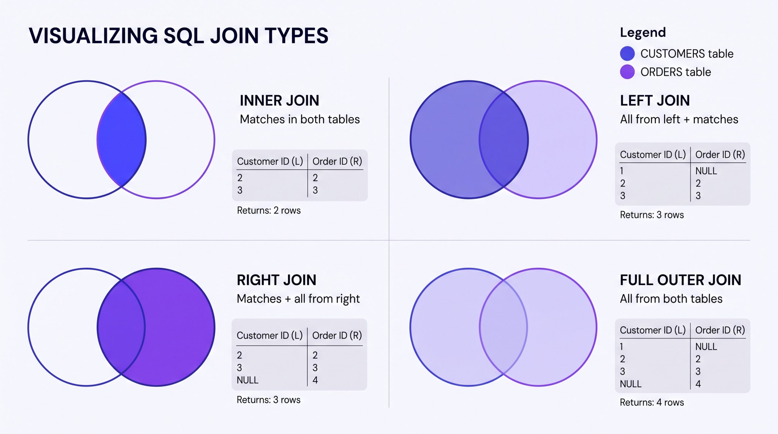
SQL Joins Venn diagram showing INNER, LEFT, RIGHT, and FULL OUTER joins with data examples and result sets

Each JOIN type returns different combinations of rows from both tables.

INNER JOIN: Only Matching Rows Beginner

Returns only rows that have matches in both tables.

SELECT 
    c.customer_id,
    c.name,
    o.order_id,
    o.amount
FROM customers c
INNER JOIN orders o ON c.customer_id = o.customer_id;

— Result: Only customers WHO HAVE PLACED ORDERS
— Customers with no orders are excluded
            

When to use: When you only care about records that exist in both tables (customers who’ve ordered, products that have been sold, etc.)

LEFT JOIN: All from Left, Matches from Right Intermediate

Returns all rows from the left table, plus matching rows from the right table. Non-matches show as NULL.

SELECT 
    c.customer_id,
    c.name,
    COUNT(o.order_id) AS total_orders
FROM customers c
LEFT JOIN orders o ON c.customer_id = o.customer_id
GROUP BY c.customer_id, c.name;

— Result: ALL CUSTOMERS with their order count
— Customers with 0 orders show 0 (or NULL becomes 0 with COALESCE)
            

When to use: When you want all records from the left table regardless of matches (all customers, all products, all employees).

RIGHT JOIN & FULL OUTER JOIN Advanced

Right JOIN is the reverse of LEFT. FULL OUTER returns all rows from both tables.

— RIGHT JOIN (uncommon, usually rewrite as LEFT)
SELECT * FROM orders o
RIGHT JOIN customers c ON o.customer_id = c.customer_id;

— FULL OUTER JOIN (rarely needed, not supported in MySQL)
SELECT * FROM customers c
FULL OUTER JOIN orders o ON c.customer_id = o.customer_id;
            

Pro tip: Most SQL databases don’t support RIGHT or FULL OUTER. Just flip your LEFT JOIN around instead.

Window Functions: The Secret Weapon Advanced

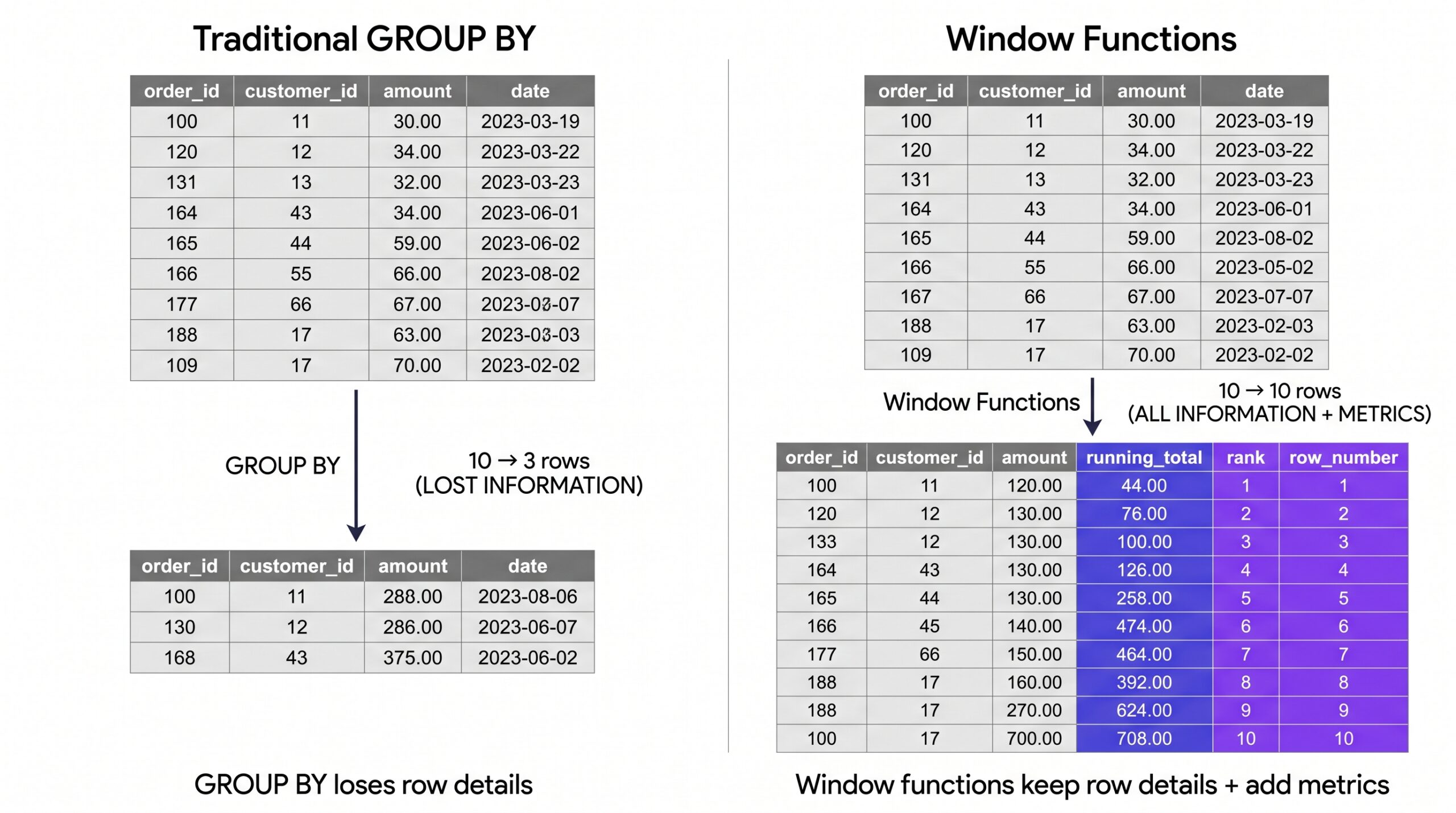
Window functions are what separates junior analysts from ones who solve complex problems. They let you calculate metrics without collapsing your data with GROUP BY.

The Game-Changing Difference

Traditional GROUP BY: Collapses rows. You lose detail.

SELECT 
    category,
    SUM(amount) AS total_sales
FROM sales
GROUP BY category;

— Result: 3 rows (one per category)
— You’ve lost all individual sale information
            

Window Functions: Adds metrics to every row. You keep detail.

SELECT 
    sale_id,
    amount,
    category,
    SUM(amount) OVER (PARTITION BY category) AS category_total
FROM sales;

— Result: 10,000 rows (all original sales)
— PLUS a new column showing category total for each row
            

Essential Window Functions for Analysts

RANK() & ROW_NUMBER() – Find top performers, detect duplicates

SELECT 
    employee_id,
    salary,
    department,
    RANK() OVER (PARTITION BY department ORDER BY salary DESC) AS rank_in_dept,
    ROW_NUMBER() OVER (PARTITION BY department ORDER BY salary DESC) AS row_num
FROM employees;

— Returns: Top earners in each department with their ranking
— RANK: ties get same rank, next rank skips (1, 1, 3)
— ROW_NUMBER: ties get different numbers (1, 2, 3)
            

LEAD() & LAG() – Compare current row to previous/next row

SELECT 
    order_date,
    amount,
    LAG(amount) OVER (ORDER BY order_date) AS prev_order_amount,
    LEAD(amount) OVER (ORDER BY order_date) AS next_order_amount,
    amount – LAG(amount) OVER (ORDER BY order_date) AS change_from_prev
FROM orders
ORDER BY order_date;

— Useful for: Detecting trends, comparing consecutive periods
            

Running SUM/AVG – Calculate cumulative totals

SELECT 
    order_date,
    amount,
    SUM(amount) OVER (ORDER BY order_date 
        ROWS BETWEEN UNBOUNDED PRECEDING AND CURRENT ROW) AS cumulative_sales
FROM orders;

— Shows: Monthly revenue + running total through that month
            

🎯 Analyst Secret

Master RANK(), ROW_NUMBER(), and LEAD()/LAG(). These three window functions solve 80% of real-world analysis problems. Everything else is icing.

Subqueries vs. CTEs: Which to Use and When? Intermediate

Both let you use the results of one query as input to another. But they’re different tools for different jobs.

Subqueries: Quick, Inline Solutions

SELECT * FROM orders
WHERE customer_id IN (
    SELECT customer_id 
    FROM customers 
    WHERE signup_date >= ‘2023-01-01’
);

— Finds all orders from customers who signed up in 2023
— Subquery runs, returns customer IDs, then filters orders
            

When to use: Simple, one-off queries. Single level of nesting.

Common Table Expressions (CTEs): Readable, Reusable

WITH new_customers AS (
    SELECT customer_id, name
    FROM customers
    WHERE signup_date >= ‘2023-01-01’
),
customer_orders AS (
    SELECT 
        nc.customer_id,
        nc.name,
        COUNT(o.order_id) AS total_orders,
        SUM(o.amount) AS total_spent
    FROM new_customers nc
    LEFT JOIN orders o ON nc.customer_id = o.customer_id
    GROUP BY nc.customer_id, nc.name
)
SELECT * FROM customer_orders
ORDER BY total_spent DESC;

— Much more readable than nested subqueries
— You can reference CTEs multiple times
            

When to use: Complex queries with multiple steps. Makes code easier to read and debug.

Factor	Subquery	CTE
Readability	Hard (nested parentheses)	Easy (named blocks)
Reusability	One-time use	Can reference multiple times
Performance	Similar	Similar (databases optimize both)
Best For	Simple, single-level queries	Complex, multi-step analysis

⚠️ Reddit Question Answered

Q: “How do I clean messy data using only SQL?”

A: With CTEs and string functions. Use TRIM(), UPPER(), CASE statements, and NULL checks to clean data before analysis. It’s cleaner (literally) to clean in SQL than in Excel, because your transformation is reproducible and automated. See the Resource section for cleanup techniques.

SQL Query Optimization: Writing Fast, Efficient Queries

The Performance Problem: Why Some Queries Feel Slow

You write a query. It works. But it takes 30 seconds. Then someone asks for a slightly different result. Now it takes 2 minutes. This is where most analysts get stuck.

Here’s what separates average queries from optimized ones:

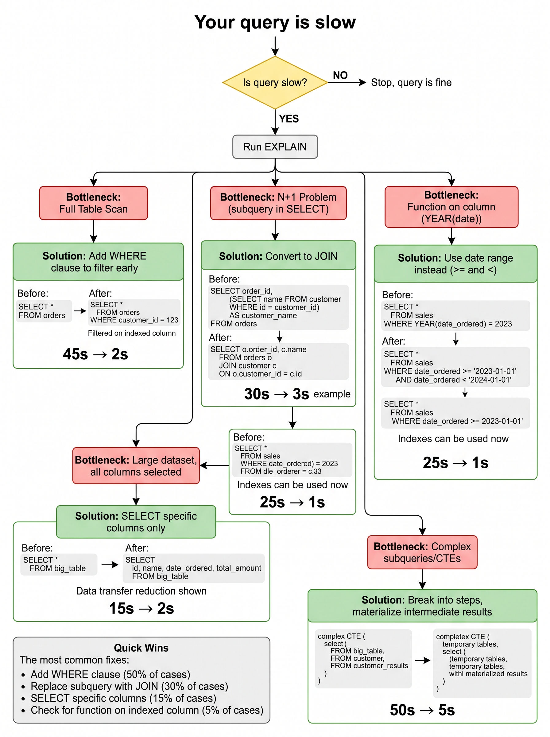
Common “Slow” Query Patterns to Avoid

❌ Don’t: Filtering on a function result

— SLOW: Extracts year from every row, then filters
SELECT * FROM orders
WHERE YEAR(order_date) = 2023;

— FAST: Uses the actual date range
SELECT * FROM orders
WHERE order_date >= ‘2023-01-01’ 
  AND order_date < '2024-01-01';
            

❌ Don’t: SELECT * when you need specific columns

— SLOW: Returns 50 columns you don’t need
SELECT * FROM large_customer_table;

— FAST: Returns only what you need
SELECT customer_id, name, email FROM large_customer_table;
            

❌ Don’t: Subqueries in SELECT for large datasets

— SLOW: Subquery runs for EVERY row
SELECT 
    order_id,
    (SELECT COUNT(*) FROM order_items WHERE order_id = o.order_id) AS item_count
FROM orders o;

— FAST: Join and aggregate once
SELECT 
    o.order_id,
    COUNT(oi.item_id) AS item_count
FROM orders o
LEFT JOIN order_items oi ON o.order_id = oi.order_id
GROUP BY o.order_id;
            

Understanding Indexes: The Speed Multiplier

An index is like a book’s index. Instead of reading every page to find mentions of “customer”, you look in the index, which has them pre-organized.

Where indexes exist (you can’t control this, but good to know):

Primary Keys – Always indexed. Fastest lookups.
Foreign Keys – Usually indexed (but not always).
High-selectivity columns – Columns where most values are unique (IDs, emails).

How to write queries that use indexes:

— GOOD: Filters on indexed column (primary key)
SELECT * FROM customers WHERE customer_id = 42;
Result: Lightning fast (milliseconds)

— GOOD: Filters on indexed column (email, unique)
SELECT * FROM customers WHERE email = ‘user@example.com’;
Result: Very fast (uses index)

— SLOW: Filters on unindexed column or with a function
SELECT * FROM customers WHERE name LIKE ‘%Smith%’;
Result: Slow (scans every row)
            

The Real-World Optimization Workflow

Step 1: Write the query correctly first – Don’t optimize prematurely.

Step 2: Run it and check execution time – Is it actually slow?

Step 3: Use EXPLAIN to see the plan – What’s taking time?

EXPLAIN SELECT * FROM orders WHERE order_date >= ‘2023-01-01’;

— Shows you which tables are scanned, whether indexes are used, etc.
— Look for “Full Table Scan” (bad) vs “Index Seek” (good)
            

Step 4: Fix the bottleneck – Add WHERE clause, use JOIN instead of subquery, etc.

🤔 Reddit Question Answered

Q: “When should I move from SQL to Python?”

A: When SQL can’t do what you need efficiently. SQL excels at: filtering, aggregating, joining. Python excels at: complex transformations, machine learning, statistical testing. Use SQL to get 80% of the way there, then Python for the remaining 20% if needed. In most jobs, 95% of your work stays in SQL.

Advanced SQL Patterns That Solve Real Problems

Detecting Duplicates & Data Quality Issues

— Find duplicate customers (same email signed up twice)
SELECT email, COUNT(*) as count
FROM customers
GROUP BY email
HAVING COUNT(*) > 1;

— Find orders with no matching customer (referential integrity issue)
SELECT o.order_id, o.customer_id
FROM orders o
LEFT JOIN customers c ON o.customer_id = c.customer_id
WHERE c.customer_id IS NULL;

— Find rows with missing required data
SELECT * FROM orders
WHERE customer_id IS NULL 
   OR order_date IS NULL 
   OR amount IS NULL;
            

Cohort Analysis: Comparing Customer Groups

Cohort analysis groups customers by signup month, then tracks their behavior over time.

WITH customer_cohorts AS (
    SELECT 
        customer_id,
        DATE_TRUNC(‘month’, signup_date) AS cohort_month
    FROM customers
),
first_order AS (
    SELECT 
        cc.customer_id,
        cc.cohort_month,
        DATE_TRUNC(‘month’, MIN(o.order_date)) AS first_order_month
    FROM customer_cohorts cc
    LEFT JOIN orders o ON cc.customer_id = o.customer_id
    GROUP BY cc.customer_id, cc.cohort_month
)
SELECT 
    cohort_month,
    EXTRACT(MONTH FROM first_order_month – cohort_month) AS months_to_first_order,
    COUNT(*) AS customer_count
FROM first_order
GROUP BY cohort_month, EXTRACT(MONTH FROM first_order_month – cohort_month)
ORDER BY cohort_month, months_to_first_order;

— Shows: Which signup month, how many months until they ordered
— Reveals if recent customers are slower to convert
            

Calculating Metrics Like Churn & Retention

Comparison of GROUP BY vs Window Functions showing how window functions keep detail while adding metrics

Window functions keep all rows while adding calculated metrics—GROUP BY collapses them.

— Monthly churn: Customers who ordered last month but not this month
WITH monthly_activity AS (
    SELECT 
        customer_id,
        DATE_TRUNC(‘month’, order_date)::date AS month
    FROM orders
),
customer_months AS (
    SELECT DISTINCT customer_id, month
    FROM monthly_activity
),
with_prev_month AS (
    SELECT 
        customer_id,
        month,
        LAG(month) OVER (PARTITION BY customer_id ORDER BY month) AS prev_month
    FROM customer_months
)
SELECT 
    month,
    COUNT(DISTINCT customer_id) AS active_customers,
    SUM(CASE WHEN prev_month IS NOT NULL THEN 1 ELSE 0 END) AS retained,
    SUM(CASE WHEN prev_month IS NULL THEN 1 ELSE 0 END) AS new
FROM with_prev_month
GROUP BY month
ORDER BY month;
            

Common Questions: Mastering SQL in Practice

Q: What is the biggest difference between learning SQL and using it at work?

A: Learning SQL, you write perfect queries from scratch. At work, you inherit broken queries and need to debug them. You spend 70% of your time understanding someone else’s code, 30% writing new code.

The skill that matters: Reading others’ queries quickly and fixing them. Take existing queries apart. Understand every JOIN. See if there’s a bug. This is how you actually learn fast at a job.

⚠️ Related Reading

To avoid costly mistakes early, read our guide on common SQL mistakes every beginner makes and how to avoid them.

Q: How do I practice SQL query optimization for interviews?

A: Use HackerRank SQL challenges or LeetCode database problems. They show execution time. Write a solution, optimize it, see if the optimization helped.

Practice pattern:

Write working query
Check execution time
Rewrite with different approach
Compare times
Understand why one was faster

Q: SQL vs. Python: When to use which for Data Analysis?

A: Use SQL for getting data. Use Python for understanding data.

Task	SQL	Python
Filter & aggregate data	✅ Excellent	⚠️ Overkill
Join multiple tables	✅ Built for this	⚠️ Requires more code
Statistical analysis	❌ Limited	✅ Excellent (pandas, scipy)
Machine learning	❌ Not possible	✅ Excellent (scikit-learn)
Data cleaning	✅ String functions work well	✅ More flexible with pandas
Visualization	❌ Not designed for it	✅ Excellent (matplotlib, seaborn)

Rule of thumb: If you’re querying a database, use SQL. If you’re manipulating results or building models, use Python.

Q: What are the most important window functions to master?

Master these 4 in this order:

ROW_NUMBER() – Rank rows, find top N per group
LAG() & LEAD() – Compare row to previous/next
SUM() OVER – Running totals
RANK() – Handle ties explicitly

Everything else is nice-to-have. These four solve 90% of real problems.

Resources: Where to Learn & Practice SQL

SQL learning has three components: understanding syntax, understanding patterns, and understanding databases. Here are the best resources for each.

🎯 Practice Platforms

Maven Analytics Data Playground

Best for: Real datasets with business context. Actually fun.

What you get: Real-world datasets ready to query. SQL editor built in. Clear problem statements.

Cost: Free to start, premium content available

Visit Maven Analytics →

LeetCode Database Problems

Best for: Interview preparation. Problem-solving practice.

What you get: 200+ SQL problems from easy to hard. Solutions and discussion. Execution time feedback.

Cost: Free tier covers most problems

Visit LeetCode →

HackerRank SQL Challenge

Best for: Building confidence with fundamentals. Good progression from easy to hard.

What you get: 70+ problems, instant feedback, community solutions

Cost: Completely free

Visit HackerRank →

📚 Learning Resources

Mode Analytics SQL Tutorial

Best for: Understanding SQL concepts interactively. Excellent explanations.

What you get: Free SQL course with a real database to query. Clear, progressive lessons.

Cost: Free

Visit Mode Analytics →

Window Functions Documentation

Best for: Reference when building complex queries. Database-specific syntax.

Database-specific links:

Cost: Free (official docs)

🏆 Advanced Reading

“Use The Index, Luke!” – Database Indexing Guide

Best for: Understanding how databases actually work under the hood

Visit Use The Index, Luke →

Reddit Communities for Help

Best for: Getting help when you’re stuck

r/SQL – 100k+ members, very helpful
r/dataanalysis – Career and skills questions
r/learnprogramming – General programming help

Cost: Free

Decision tree flowchart for optimizing slow SQL queries, showing bottleneck identification and solution paths

Follow this decision tree when you encounter slow queries—systematically identify the bottleneck and apply the right fix.

Conclusion: Your Path to SQL Mastery

Here’s what separates average SQL analysts from great ones:

Average: Knows SELECT, WHERE, GROUP BY. Writes queries that work.

Great: Understands why queries work. Writes queries that are fast, readable, and maintainable.

You now have the knowledge. The only step left is to practice.

Your 30-Day SQL Mastery Plan

Week 1: Master the core query structure. Complete 10 problems on Maven Analytics focusing on SELECT, WHERE, GROUP BY, HAVING.

Week 2: Master JOINs. Build queries combining 2-3 tables. Complete INNER JOIN and LEFT JOIN problems.

Week 3: Learn Window Functions. Write 5 queries using ROW_NUMBER(), LAG(), and SUM() OVER().

Week 4: Optimize & Debug. Take your previous queries, use EXPLAIN, find the slow one, optimize it, compare times.

That’s it. One month. Deliberate practice. You’ll be dangerous.

Level Up Your SQL Skills

SQL mastery doesn’t happen in tutorials. It happens when you build real projects with real data.

Join The Lab Newsletter and get SQL challenges delivered to your inbox every week. Real problems, real solutions, real learning.

Plus: Early access to our SQL project walkthroughs and optimization tips.

Subscribe to The Lab →